

Minimizing Errors: The Journey of the Cost Function in Linear Regression - A Concrete Example of Seeking Global Minima


Table of contents
- INTRODUCTION
- DIFFERENCE BETWEEN ERROR FUNCTION AND COST FUNCTION
- DIFFERENCE BETWEEN GLOBAL MINIMA AND LOCAL MINIMA
- COST FUNCTION FOR LINEAR REGRESSION
- WHAT IS GRADIENT DESCENT?
- WHAT IS THE LEARNING RATE?
- DERIVATION OF GRADIENT DESCENT IN LINEAR REGRESSION
- STEPS FOLLOWED IN GRADIENT DESCENT
- CODE FOR GRADIENT DESCENT
- CONCLUSION
INTRODUCTION
Welcome to our blog post, where we embark on a journey to understand how the cost function in linear regression works. In this article, we will dive into the fascinating world of optimization and global minima, using a concrete numerical example to illustrate the concepts. By unraveling the inner workings of the cost function, we will demystify how it drives the process of error minimization in linear regression.
DIFFERENCE BETWEEN ERROR FUNCTION AND COST FUNCTION
| Error Function | Cost Function |
| Primarily used in the context of single examples or predictions. | Typically used in the context of training a machine learning model on a dataset. |
| Measures the discrepancy between the predicted output and the actual output for a single data point. | Quantifies the overall performance or fit of a model on an entire dataset. |
| Examples include Mean absolute error (MAE), Mean squared error (MSE), or root mean squared error (RMSE). | Examples include the Sum of Mean Squared Error (MSE), or log loss (for classification tasks). |
| The goal is to minimize the error for each individual prediction. | The goal is to find model parameters that minimize the overall cost across the entire dataset. |
NOTE:
The terms "error function" and "cost function" are often used interchangeably, depending on the context and specific application.
However, the key distinction lies in their primary usage: error functions focus on individual predictions, while cost functions are used to optimize models on datasets.
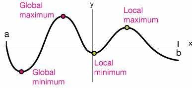
DIFFERENCE BETWEEN GLOBAL MINIMA AND LOCAL MINIMA
| Global Minima | Local Minima |
| Represents the lowest point of the entire function. | Refers to the lowest point within a specific region or neighborhood of the function. |
| Corresponds to the absolute lowest value of the function. | Represents a relatively low value compared to nearby points but may not be the absolute lowest value in the entire function. |
This figure gives you a clear idea.
NOTE:
In optimization problems, finding the global minimum is typically the ultimate goal as it guarantees the best possible solution.
However, local minima can be problematic because they can trap optimization algorithms, leading to suboptimal solutions if the global minimum is not reached.
COST FUNCTION FOR LINEAR REGRESSION
In linear regression, the most commonly used error function is the mean squared error (MSE).
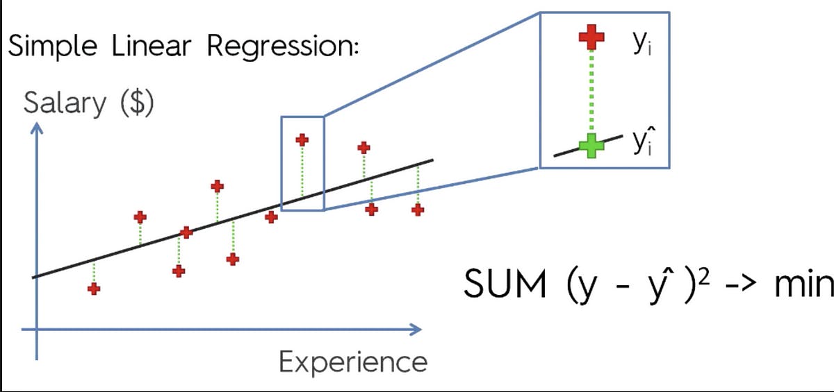
$$MSE = (1/n) * Σ(y - ŷ)^2$$
where:
n is the number of observations in the dataset,
y represents the actual values of the target variable,
ŷ represents the predicted values of the target variable.
WHAT IS GRADIENT DESCENT?
Gradient descent is an optimization algorithm used to minimize a function iteratively by adjusting its parameters in the direction of the negative gradient.
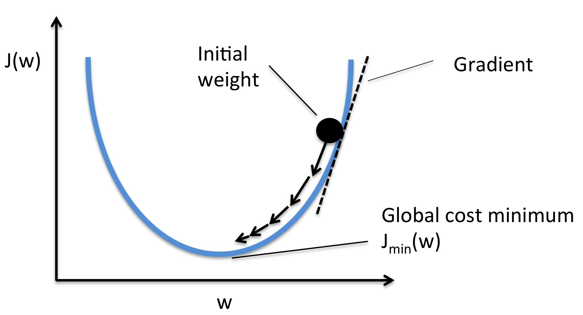
FORMULA
$$xᵢ₊₁ = xᵢ - α * ∇f(xᵢ)$$
where:
xᵢ is the current parameter value at iteration i,
α (alpha) is the learning rate that controls the step size,
∇f(xᵢ) is the gradient of the function f(x) concerning x, representing the direction and magnitude of the steepest descent.
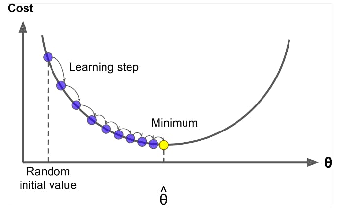
WHAT IS THE LEARNING RATE?
The learning rate in gradient descent is the step size or rate at which the model parameters are adjusted during each iteration.
DERIVATION OF GRADIENT DESCENT IN LINEAR REGRESSION
W.K.T Cost function
$$MSE = (1/n) * Σ(y - ŷ)^2$$
W.K.T Equation of simple linear regression
$$ŷ=mx+c$$
Step 1: Let us take the initial point and point which is at the next step.
Equation 1: The slope between the points
$$m2=m1-L*Dm$$
Equation 2: The intercept between the points
$$c2=c1-L*Dc$$
Here,
L - Learning Rate
m1,m2 - Slope of the points
Dm - Partial derivative of cost function concerning m
Dc -Partial derivative of cost function concerning c
Step 2: Find Dm
$$∂(MSE)/∂m=∂((1/n) * Σ(y - ŷ)^2)/∂m$$
Substitute ŷ in the above equation
$$∂(MSE)/∂m=∂((1/n) * Σ(y - (mx+c))^2)/∂m$$
(a+b)^2 Formula
$$∂(MSE)/∂m=(1/n) * ∂(Σ(y^2 +(mx+c)^2-2y(mx+c))/∂m$$
Expanding
$$∂(MSE)/∂m=(1/n) * Σ(∂(y^2 +(mx)^2+c^2+2mxc-2mxy-2yc))/∂m$$
After differentiation, we get finally
$$Dm=-2/n*Σx(y-(mx+c))$$
Step 3: Find Dc
The partial derivative of MSE concerned with c
$$∂(MSE)/∂c=(1/n) * Σ(∂(y^2 +(mx)^2+c^2+2mxc-2mxy-2yc))/∂c$$
Finally, we get,
$$Dc=-2/n*Σ(y-(mx+c))$$
Step 3: Finally substitute Dm and Dc values in the equations
we get,
$$m2=m1-L*(-2/n*Σx(y-(mx+c)))$$
$$c2=c1-L*(-2/n*Σ(y-(mx+c)))$$
Step 4: This is the iterative process until it finds global minima(ideally 0) by simultaneously updating m and c for the given dataset
Hence in general,
Formulas
$$m=m+L*(2/n*Σxᵢ(yᵢ-(mxᵢ+cᵢ)))$$
$$c=c+L*(2/n*Σ(yᵢ-(mxᵢ+cᵢ)))$$
STEPS FOLLOWED IN GRADIENT DESCENT
Step1: Define the cost function
Step2: Derivative of the Cost function
Step3: Initialize lr m and c randomly
Step 4: Repeat until convergence by using the derived formula, simultaneously updating m and c.
CODE FOR GRADIENT DESCENT
#loss=(y-yhat)**2/N

import numpy as np

#initialize parameter
#for example
x=np.random.randn(10,1)
y=2*x+np.random.rand()
#initially slope and intercept
m=0.0
c=0
#let say our model leraning rate 0.1
learning_rate=0.01
#create gradient descent
def gradient_descent_linear_regression(x,y,m,c,learning_rate):
    #partial derivative
    dldm=0
    dldc=0
    #number samples in data
    N=x.shape[0]
    for xi,yi in zip(x,y):
        dldm+=-2*xi*(yi-(m*xi+c))
        dldc+=-2*(yi-(m*xi+c))

        #make update to slope and intercept
        m=m-learning_rate*(1/N)*dldm
        c=c-learning_rate*(1/N)*dldm
    return m,c

#iteratively update
for epoch in range(3):
    m,c=gradient_descent_linear_regression(x,y,m,c,learning_rate)
    yhat=m*x+c
    loss=np.divide(np.sum((y-yhat)**2),x.shape[0])
    print(f"for{epoch} Loss is {loss},slope{m},intercept{c}")
OUTPUT
for0 Loss is 3.7289331846009013,slope[0.23119888],intercept[0.23119888]
for1 Loss is 2.8466961593922298,slope[0.43515356],intercept[0.43515356]
for2 Loss is 2.2170477365170203,slope[0.61507449],intercept[0.61507449]
NOTE: For the 3 iterations in the above example for random data points we obtain
slope m=0.61
intercept=0.61 where the loss is minimum.
This is the mathematical intuition behind gradient descent in linear regression.Based on the loss it will compute the optimal slope and intercept for the data set.
CONCLUSION
Gradient descent plays a crucial role in the field of linear regression by enabling the optimization of model parameters to minimize the cost function. Through iterative updates, the algorithm guides the model toward the best-fitting line that minimizes the overall difference between predicted and actual values. By leveraging the power of gradient descent, linear regression models can effectively learn from data and make accurate predictions. Understanding and implementing gradient descent in linear regression empowers practitioners to unlock the full potential of this widely-used and essential algorithm in the realm of machine learning.
Hope you enjoyed the learning !!!
Stay tuned !!!
Thank you !!!