

Unleashing the Power of Polynomial Regression: A Comprehensive Guide


Table of contents
- INTRODUCTION
- POLYNOMIAL REGRESSION
- POLYNOMIAL EQUATION
- TYPES OF POLYNOMIAL REGRESSION
- QUADRATIC REGRESSION
- STREAMLINING QUADRATIC REGRESSION CALCULATIONS
- MATHEMATICAL EXAMPLE FOR QUADRATIC REGRESSION
- EXAMPLE CODE FOR POLYNOMIAL REGRESSION
- EXAMPLE OF OVER-FITTING AND UNDERFITTING IN POLYNOMIAL REGRESSION
- WHEN TO USE POLYNOMIAL REGRESSION?
- CONCLUSION
INTRODUCTION
In the realm of data analysis and machine learning, finding patterns and uncovering relationships between variables is of utmost importance. While linear regression serves as a fundamental tool for modeling such relationships, it may fall short when faced with complex, nonlinear data. Enter polynomial regression—a versatile technique that allows us to capture nonlinear trends and achieve greater accuracy in our predictions.
In this blog post, we will delve into the world of polynomial regression and explore its potential to unlock valuable insights from our data. Whether you're a beginner taking your first steps into regression analysis or an experienced data scientist seeking to expand your modeling toolbox, this guide will provide you with a solid foundation to harness the power of polynomial regression effectively.
POLYNOMIAL REGRESSION
Polynomial regression is a form of regression analysis that extends the capabilities of linear regression by allowing for nonlinear relationships between the independent variable(s) and the dependent variable. While linear regression assumes a linear relationship between variables, polynomial regression can capture more complex relationships by introducing polynomial terms of higher degrees.
POLYNOMIAL EQUATION
In polynomial regression, the relationship between the independent variable(s) and the dependent variable is modeled as an nth-degree polynomial function. The polynomial equation takes the form:
$$y = β0 + β1x + β2x² + β3x³ + ... + βnxⁿ$$
where:
y represents the dependent variable,
x represents the independent variable,
β₀, β₁, β₂, ..., βₙ are the coefficients that determine the shape and magnitude of the polynomial terms.
NOTE:
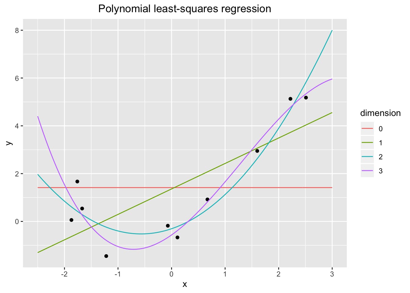
The choice of the degree of the polynomial, denoted by n, depends on the complexity of the relationship between the variables and the data at hand.
By increasing the degree of the polynomial, the model can fit the data more closely and capture intricate nonlinear patterns.
However, a higher degree polynomial may also introduce overfitting if the model becomes too complex and starts capturing noise rather than the underlying signal.
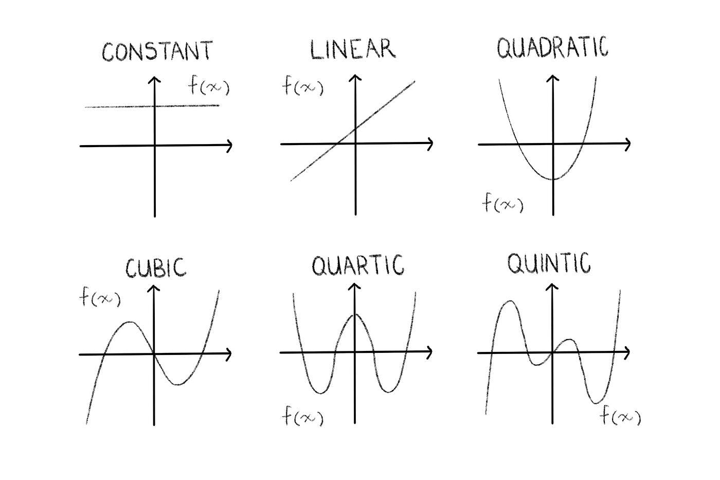
TYPES OF POLYNOMIAL REGRESSION
Linear Regression (Degree 1)
Quadratic Regression (Degree 2)
Higher Degree Polynomial Regression (Degree > 2)
QUADRATIC REGRESSION
Quadratic polynomial regression, also known as quadratic regression, is a specific type of polynomial regression where the relationship between the independent variable and the dependent variable is modeled using a quadratic function.
EQUATION
$$y = β0 + β1x + β2x²$$
STREAMLINING QUADRATIC REGRESSION CALCULATIONS
To solve Quadratic regression we have to solve a system of three equations:
They are:
EQUATION 1:
$$∑y =nβ0+β1∑x+β2∑x^2$$
where,
n-Number of data points in given data
EQUATION 2:
$$∑xy =β0∑x+β1∑x^2+β2∑x^3$$
EQUATION 3:
$$∑x^2y =β0∑x^2+β1∑x^3+β2∑x^4$$
By solving the above equation we will get β0,β1,β2
Substitute β0,β1,β2 in the Quadratic equation.
MATHEMATICAL EXAMPLE FOR QUADRATIC REGRESSION
Obtain the regression equation for degree=2 for the given data points
| x | 3 | 4 | 5 | 6 | 7 |
| y | 2.5 | 3.2 | 3.8 | 6.5 | 12 |
Solution:
Step 1: Calculating ∑x, ∑y, ∑x^2, ∑x^3, ∑x^4, ∑xy, ∑x^2y
Here, The total number of data points is 5.
hence n=5
| x | y | x^2 | x^3 | x^4 | xy | x^2y |
| 3 | 2.5 | 9 | 27 | 81 | 7.5 | 22.5 |
| 4 | 3.2 | 16 | 64 | 256 | 12.8 | 51.2 |
| 5 | 3.8 | 25 | 125 | 625 | 19 | 95 |
| 6 | 6.5 | 36 | 216 | 1296 | 39 | 234 |
| 7 | 12 | 49 | 343 | 2401 | 80.5 | 563.5 |
| ∑x=25 | ∑y=27.5 | ∑x^2=135 | ∑x^3=775 | ∑x^4=4659 | ∑xy=158.8 | ∑x^2y=966.2 |
Step 2: Substituting the values in a system of 3 equations
EQUATION 1:
$$27.5 =(5)β0+β1(25)+β2(135)$$
EQUATION 2:
$$158.8=β0(25)+β1(135)+β2(775)$$
EQUATION 3:
$$966.2 =β0(135)+β1(775)+β2(4659)$$
By solving the above three equations by matrix method we get
β0=12.4285714
β1=-5.5128571
β2=0.7642857
Step 4: Substituting β0, β1, β2 in quadratic equation
w.k.t quadratic equation is
$$y = β0 + β1x + β2x²$$
Obtained equation is
$$y = 12.4285714 -5.5128571x + 0.7642857x²$$
EXAMPLE CODE FOR POLYNOMIAL REGRESSION
The code using the above data points in mathematical calculation
import numpy as np
import pandas as pf
import matplotlib.pyplot as plt
from sklearn.linear_model import LinearRegression
from sklearn.preprocessing import PolynomialFeatures
#data
x=np.array([3,4,5,6,7])
y=np.array([2.5,3.2,3.8,6.5,12])
#reshaping indpendent variable
x=x.reshape(-1,1)
#how curve fit from degree 1 to 2
for i in range(1,3):
    polynomial=PolynomialFeatures(degree=i)
    x_poly=polynomial.fit_transform(x)
    polynomial.fit(x_poly,y)
    linear=LinearRegression()
    linear.fit(x_poly,y)
    y_pred=linear.predict(x_poly)
    plt.scatter(x,y,color='blue')
    plt.plot(x,y_pred,color='red')
    plt.show()
OUTPUT
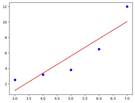
Output for degree=1:
Output for degree=2:
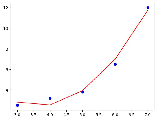
See, how increasing the degree from 1 to 2 helps the model to learn more effectively.
Note: For degree=1 the model is underfit.
EXAMPLE OF OVER-FITTING AND UNDERFITTING IN POLYNOMIAL REGRESSION
import numpy as np
import pandas as pf
import matplotlib.pyplot as plt
from sklearn.linear_model import LinearRegression
from sklearn.preprocessing import PolynomialFeatures
#data
x = np.array([1, 5, 3, 2, 6])
y = np.array([2, 6, 10, 20, 30])
#reshaping indpendent variable
x=x.reshape(-1,1)
#model performance from degree 1 to 4
for i in range(1,5):
    polynomial=PolynomialFeatures(degree=i)
    x_poly=polynomial.fit_transform(x)
    print('Polynomial Features',x_poly)
    polynomial.fit(x_poly,y)
    linear=LinearRegression()
    linear.fit(x_poly,y)
    y_pred=linear.predict(x_poly)
    plt.scatter(x,y,color='blue')
    plt.plot(x,y_pred,color='red')
    plt.show()
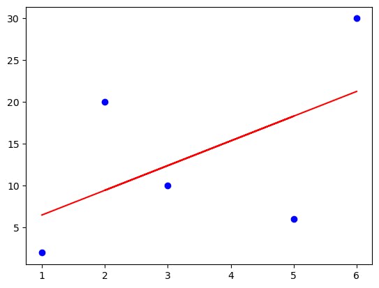
OUTPUT
Underfitting by the model for the data points at
degree=1:
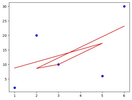
degree=2:
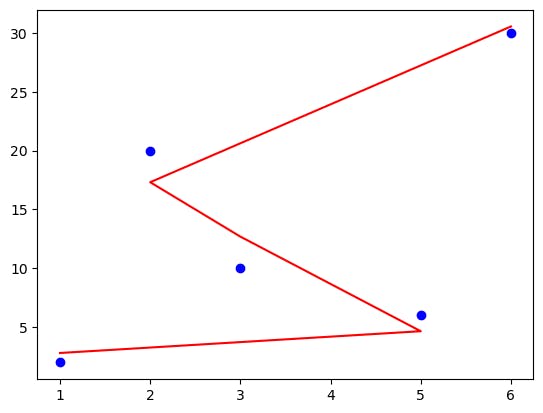
Good performance of the model at the
degree=3:
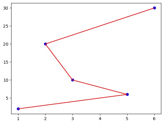
Overfitting by the model at
degree=4:
WHEN TO USE POLYNOMIAL REGRESSION?
| Situation | Polynomial Regression Usage |
| Nonlinear Relationships | When the relationship between variables exhibits curvature or nonlinearity, polynomial regression can capture these complex patterns. |
| U-Shaped or Inverted U-Shaped Relationships | Polynomial regression is effective in modeling relationships that follow a U-shaped or inverted U-shaped curve. |
| Flexibility in Modeling | Polynomial regression provides greater flexibility than linear regression by allowing for higher-degree polynomial terms, enabling a better fit to the data. |
| Interaction Effects | Polynomial regression can capture interaction effects between variables, where the relationship between them changes with different values of the variables. |
| Limited Prior Knowledge of the Relationship | When there is limited prior knowledge or theory about the underlying relationship, polynomial regression can be used as a more exploratory modeling approach. |
| Data Visualization and Interpretability | Polynomial regression can help visualize and interpret complex relationships, as the higher-degree terms allow for more detailed insights into the data. |
| The trade-Off between Bias and Variance | By adjusting the degree of the polynomial, one can find an optimal trade-off between bias and variance in the model, depending on the dataset and desired level of complexity. |
| ***Warning: Overfitting | Be cautious when using high-degree polynomials, as they can lead to overfitting, capturing noise rather than true patterns. Regularization techniques may be necessary to mitigate this. |
CONCLUSION
In conclusion, polynomial regression offers a powerful tool for modeling nonlinear relationships and capturing complex patterns in the data. By extending beyond linear regression, it provides flexibility in fitting curves, capturing U-shaped relationships, and exploring interaction effects. However, caution should be exercised to avoid overfitting and ensure the appropriate degree of the polynomial is chosen based on the data characteristics.
Refer this to for Linear regression and for solving system of equations
HOPE YOU ENJOYED READING IT!!!
STAY TUNED !!!
SUPPORT MY BLOG !!!
THANKYOU !!!