Connecting the Dots: Exploring the Magic of Interpolation in Data Science


Table of contents
- INTRODUCTION
- SIMPLE LINEAR INTERPOLATION
- NUMERICAL EXAMPLE FOR LINEAR INTERPOLATION
- IMPLEMENTATION OF LINEAR INTERPOLATION
- BI-LINEAR INTERPOLATION
- NUMERICAL EXAMPLE FOR BILINEAR INTERPOLATION
- IMPLEMENTATION OF BI-LINEAR INTERPOLATION
- POLYNOMIAL INTERPOLATION-LAGRANGE METHOD
- NUMERICAL EXAMPLE FOR POLYNOMIAL INTERPOLATION- LAGRANGE METHOD
- POLYNOMIAL INTERPOLATION-NEWTON'S DIVIDED DIFFERENCE METHOD
- NUMERICAL EXAMPLE FOR POLYNOMIAL INTERPOLATION-NEWTON'S DIVIDED DIFFERENCE METHOD
- IMPLEMENTATION FOR POLYNOMIAL INTERPOLATION
- WHEN TO USE WHICH INTERPOLATION?
- CONCLUSION
INTRODUCTION
Welcome to our blog, where we embark on a captivating exploration of the art and science of interpolation. In the realm of data science, interpolations serve as a powerful tool, enabling us to fill in the gaps, predict missing values, and extract hidden patterns from our data. Join us as we unravel the intricacies of interpolation techniques, uncover their real-world applications, and witness the remarkable impact they have on data analysis and decision-making. Get ready to unlock the potential of interpolation and unleash the true potential of your data.

SIMPLE LINEAR INTERPOLATION
Linear interpolation is a technique that estimates values between two known data points by assuming a straight-line relationship, allowing for the approximation of intermediate values based on the slope and distance between the known points.
FORMULA

NUMERICAL EXAMPLE FOR LINEAR INTERPOLATION
Find the value of 2.4 by linear interpolation using the given data
| x | 2 | 3 |
| y | 4 | 9 |
Solution
To find target value y when x=2.4
w.k.t
$$y=y1+((y2-y1)/(x2-x1))*(x-x1)$$
From the given data
x=2.4 lies between (2,3)
hence,
x1=2,x2=3
y1=4,y2=9
substitute in the formula
we get for x=2.4
Value of y is
$$y=6$$
IMPLEMENTATION OF LINEAR INTERPOLATION
import numpy as np

def linear_interpolation(x_known, y_known, x_interp):
    # Perform linear interpolation
    y_interp = np.interp(x_interp, x_known, y_known)
    return y_interp

# Example usage
x_known = [2,3]
y_known = [4,9]
x_interp = [2.4]

y_interp = linear_interpolation(x_known, y_known, x_interp)
print(y_interp)
OUTPUT
[6.]
BI-LINEAR INTERPOLATION
Bilinear interpolation is a method that estimates values within a grid or a rectangular area by considering the weighted average of the surrounding four known data points, taking into account both the distance and the intensity of the points.
FORMULA

From the fig
**Step 1:**Interpolating in x direction(keep y1 constant)
f(x,y1)={((x2-x)/(x2-x1))*f(x1,y1)}
+
{((x-x1)/(x2-x1))*f(x2,y1)}
Step 2:Interpolating in x direction(keep y2 constant)
f(x,y2)={((x2-x)/(x2-x1))*f(x1,y2)}
+
{((x-x1)/(x2-x1))*f(x2,y2)}
Step 3:Interpolating in y direction**(Keep x constant)**
f(x,y)={((y2-y)/(y2-y1))*f(x,y1)}
+
{((y-y1)/(y2-y1))*f(x,y2)}
from step 1 and 2 substitute f(x,y1) and f(x,y2) in above equation we obtain
f(x,y)=(1/((x2-x1)*(y2-y1)))*A
where A
A={(y2-y)*[(x2-x)*f(x1,y1)]+[(x-x1)*f(x2,y1)]}
+
{(y-y1)*[(x2-x)*f(x1,y2)]+[(x-x1)*f(x2,y2)]}
NUMERICAL EXAMPLE FOR BILINEAR INTERPOLATION
Suppose you have measured temperatures at several coordinates on the surface of a rectangular heated plate.
The measured temperature is given by

Solution
From the Given figure
| x | y | Temp=f(x,y) |
| x1=2 | y1=1 | f(x1,y1)=60 |
| x2=9 | y1=1 | f(x2,y1)=57.5 |
| x1=2 | y2=6 | f(x1,y2)=55 |
| x2=9 | y2=6 | f(x2,y2)=70 |
| x=7 | y=5 | f(x,y)=? |
To find
f(7,5)=?
w.k.t
f(x,y)={1/((x2-x1)*(y2-y1))}*{(y2-y)*[(x2-x)*f(x1,y1)]+[(x-x1)*f(x2,y1)]}
+
{(y-y1)*[(x2-x)*f(x1,y2)]+[(x-x1)*f(x2,y2)]}
Substitue the values from the table in the above equation we get
$$f(x,y)=f(7,5)=64.2$$
IMPLEMENTATION OF BI-LINEAR INTERPOLATION
import numpy as np
from scipy.interpolate import interp2d

# Example data
x_known = np.array([2, 9, 2, 9])
y_known = np.array([1, 1, 6, 6])
z_known = np.array([60, 57.5, 55, 70])

# Create the interpolation function
interpolator = interp2d(x_known, y_known, z_known, kind='linear')

# Example interpolation
x_interp = 7
y_interp = 5
interpolated_value = interpolator(x_interp, y_interp)

print(interpolated_value)
OUTPUT
[64.21428571]
POLYNOMIAL INTERPOLATION-LAGRANGE METHOD
Lagrange polynomial interpolation is a technique that constructs a polynomial function by using a set of known data points. The resulting polynomial passes through each of the data points, allowing for the estimation of values at intermediate positions within the range of the known data.
FORMULA

NOTE:
If there are n+1 ordered pairs then the lowest degree of polynomial that connect these pair of points is n.
Example for the given note,

NUMERICAL EXAMPLE FOR POLYNOMIAL INTERPOLATION- LAGRANGE METHOD
Determine value of f(7) for the given set of data using polynomial Lagrange interpolation
| x | f(x) |
| 1 | 12 |
| 5 | -26 |
| 8 | -14 |
| 10 | 37 |
Solution
The given data has 4 pairs
hence degree will be
$$n=4-1=3$$
w.k.t
Lagrange equation for polynomial of degree n=3 is

For the given table
| x | f(x) |
| x0=1 | f(x0)=12 |
| x1=5 | f(x1)=-26 |
| x2=8 | f(x2)=-14 |
| x3=10 | f(x3)=37 |
| x=7 | f(x)=? |
Substituting all the above values in the formula we obtain
$$f(7)=-25.0190476$$
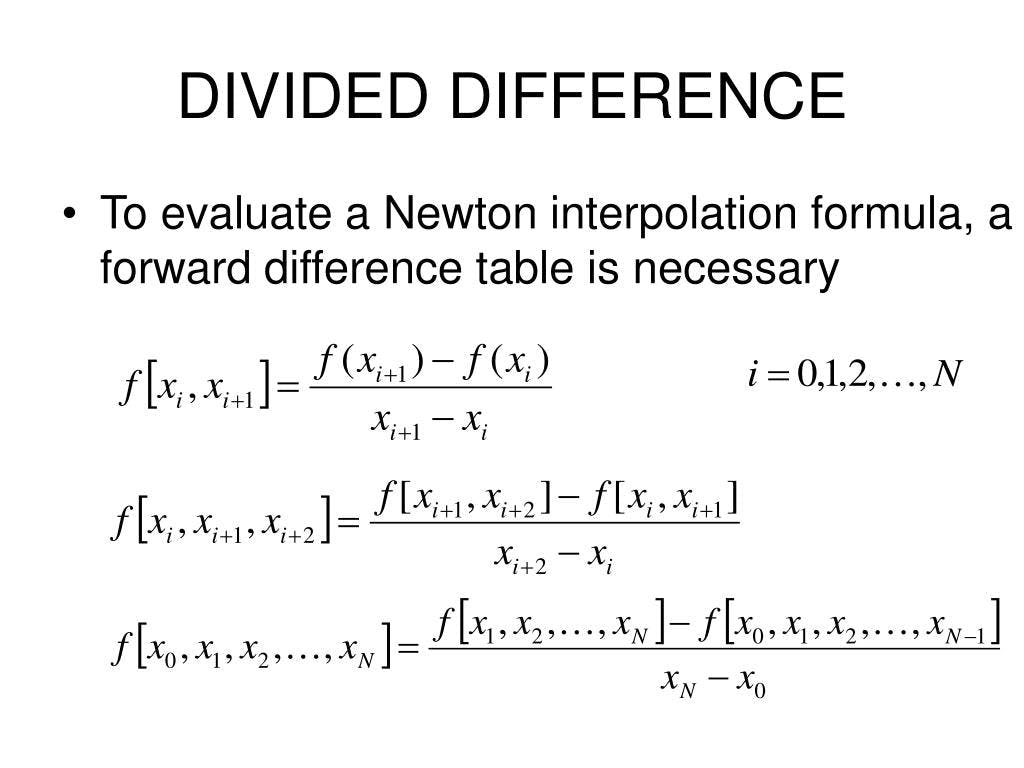
POLYNOMIAL INTERPOLATION-NEWTON'S DIVIDED DIFFERENCE METHOD
Polynomial interpolation using Newton's divided difference method is a technique that estimates values between known data points by constructing an interpolating polynomial using a divided difference table, which provides a more efficient way to evaluate the polynomial at different interpolation points.
FORMULA
$$f(x)=a0+a1(x-x0)+a2(x-x0)(x-x1)+...+an(x-x0)(x-x1)..(x-xn-1)$$
NUMERICAL EXAMPLE FOR POLYNOMIAL INTERPOLATION-NEWTON'S DIVIDED DIFFERENCE METHOD
Determine the value of f(7) for given data using Newton's difference method
| x | y | |
| 1 | 12 | |
| 5 | -26 | |
| 8 | -14 | |
| 10 | 37 |
Solution
Step 1:Tabulation method and apply the formula
(y_current-y_previous)/(x_current-x_previous)
| x | y | y' | y'' | y''' |
| x0=1 | 12 | |||
| x1=5 | -26 | -9.5 | ||
| x2=8 | -14 | 4 | 1.9285714 | |
| x3=10 | 37 | 25.5 | 4.3 | 0.2634921 |
Step 2:from the table in step 1
Diagonal elements are the coefficient i.e
$$a0=12$$
$$a1=-9.5$$
$$a2=1.9285714$$
$$a3=0.2634921$$
by substituting we obtain
$$f(x)=12-9.5(x-1)+1.9285714(x-1)(x-5)+0.2634921(x-1)(x-5)(x-8)$$
Step 3: for f(7)
$$f(7)=-25.0190484$$
IMPLEMENTATION FOR POLYNOMIAL INTERPOLATION
import numpy as np

def polynomial_interpolation(x_known, y_known, x_interp):
    coefficients = np.polyfit(x_known, y_known, len(x_known) - 1)
    y_interp = np.polyval(coefficients, x_interp)
    return y_interp

# Example usage
x_known = np.array([1, 5, 8, 10])
y_known = np.array([12, -26, -14, 37])
x_interp = np.array([7])

y_interp = polynomial_interpolation(x_known, y_known, x_interp)
print(y_interp)
OUTPUT
[-25.01904762]
WHEN TO USE WHICH INTERPOLATION?
| Interpolation Method | Scenario |
| Linear Interpolation | - When the data points form a linear pattern or trend. When the data points are evenly spaced and a simple approximation is sufficient. When estimating values between known points in a 1D dataset. When the data exhibits a linear relationship and does not have significant curvature or complexity. |
| Bilinear Interpolation | - When working with 2D data in a grid-like structure. When estimating values between known points in a rectangular grid. When the data exhibits smoothness and continuity in both dimensions. |
| Polynomial Interpolation | - When the data points do not follow a linear pattern and exhibit complex behavior. When a more accurate estimation is required between known data points. When there is a need to capture curvature or higher-order relationships in the data. When the degree of a polynomial can be chosen to fit the data well. |
CONCLUSION
In conclusion, interpolations play a crucial role in data science by providing a means to estimate values between known data points. In this blog, we explored three important interpolation methods: linear interpolation, bilinear interpolation, and polynomial interpolation using Newton's divided difference method.
Linear interpolation is suitable for data with a linear trend or evenly spaced points, while bilinear interpolation is ideal for 2D grid-like data, preserving linearity along both axes. Polynomial interpolation allows for fitting complex data patterns with higher accuracy but with increased computational complexity.
In our next blog, we will delve into some other significant interpolation techniques commonly used in the field of data science. These may include spline interpolation, Moving average etc... Stay tuned for an exploration of these advanced interpolation methods and their applications in data science.
Hope enjoyed the learning !!!
Thank you!!!