Exploring the Wonders of Probability and Statistics: A Fascinating Journey through the World of Data Science


Table of contents
- INTRODUCTION
- WHAT IS THE DEGREE OF FREEDOM?
- POPULATION vs SAMPLE
- TYPES OF POPULATION AND SAMPLE
- Population mean(μ)
- Population variance(σ^2)
- Population standard deviation(σ)
- Sample mean(x̄)
- Sample variance(s^2)
- Sample standard deviation
- MEASURE OF CENTRAL TENDENCY
- Mean
- Median
- Mode
- Example for Mean Median Mode
- Weighted Mean
- Trimmed Mean
- PERCENTILES AND QUANTILES
- MEASURE OF DISPERSION
- Range
- Variance
- Standard Deviation
- Inter Quartile Range(IQR)
- Mean Absolute Deviation
- Coefficient of variance
- SKEWNESS
- KURTOSIS
- Difference between Skewness and Kurtosis
- COVARIANCE
- CORRELATION
- Pearson correlation coefficient
- Difference between Covariance and Correlation?
- STANDARDIZATION
- NORMALIZATION
- Difference between Standardization and Normalization
- PROBABILITY DISTRIBUTION
- Probability Mass Function
- Properties of Probability Mass function
- Cumulative Distribution Function for PMF
- Probability Density Function
- Properties of the Probability density function
- Cumulative Distribution Function for PDF
- Properties of Cumulative distribution function
- Common types of Discrete probability distribution
- Bernoulli Distribution
- Binomial distribution
- Multinomial distribution
- Common types of Continuous probability distribution
- Normal Distribution
- Log-Normal Distribution
- Student's T distribution-Test
- Chi-square Distribution-Test
- TRANSFORMATION
- Logarithmic transformation
- Exponential Transformation
- Square Root Transformation
- Power Transformation
- What is heteroscedasticity?
- CONCLUSION
INTRODUCTION
Embark on an exciting journey through the captivating world of probability and statistics in data science. Discover the power of numbers as we unravel the mysteries of uncertainty, explore data patterns, and make informed decisions. Join us as we navigate the realms of probability distributions, statistical inference, and real-world applications. Get ready to unleash the full potential of probability and statistics in the captivating realm of data science. Let the adventure begin!
WHAT IS THE DEGREE OF FREEDOM?
Degrees of freedom, often represented by v or df, is the number of independent pieces of information used to calculate a statistic. It’s calculated as the sample size minus the number of restrictions.
$$df = n − 1$$
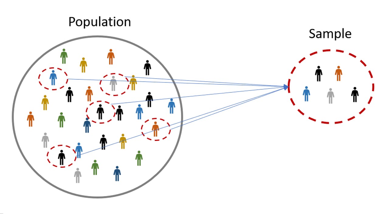
POPULATION vs SAMPLE
A population is an entire group that you want to draw conclusions about.
A sample is a specific group that you will collect data from. The size of the sample is always less than the total size of the population.
TYPES OF POPULATION AND SAMPLE

Population mean(μ)
The population mean represents the average value of a variable in the entire population.
$$μ = (Σx) / N$$
Where:
μ is the population mean.
Σx represents the sum of all individual values in the population.
N is the total number of observations in the population.
Population variance(σ^2)
The population variance measures the spread or dispersion of the data points around the population mean.
$$σ^2 = Σ((x - μ)^2) / N$$
Where:
σ^2 is the population variance.
Σ((x - μ)^2) represents the sum of squared differences between each data point (x) and the population mean (μ).
N is the total number of observations in the population.
Population standard deviation(σ)
The population standard deviation is the square root of the population variance and provides a measure of the dispersion in the population.
$$σ = √(Σ((x - μ)^2) / N)$$
Where:
σ is the population standard deviation.
Σ((x - μ)^2) represents the sum of squared differences between each data point (x) and the population mean (μ).
N is the total number of observations in the population.
Sample mean(x̄)
The sample mean represents the average value of a variable in a sample.
$$x̄ = (Σx) / n$$
Where:
x̄ is the sample mean.
Σx represents the sum of all individual values in the sample.
n is the sample size (the number of observations in the sample).
Sample variance(s^2)
The sample variance estimates the spread or dispersion of the data points around the sample mean.
$$s^2 = Σ((x - x̄)^2) / (n - 1)$$
Where:
s^2 is the sample variance.
Σ((x - x̄)^2) represents the sum of squared differences between each data point (x) and the sample mean (x̄).
n is the sample size (the number of observations in the sample).
NOTE:(n - 1) is used to account for the degrees of freedom in the sample.
Sample standard deviation
The sample standard deviation is the square root of the sample variance and provides a measure of the dispersion in the sample.
$$s = √(Σ((x - x̄)^2) / (n - 1))$$
Where:
s is the sample standard deviation.
Σ((x - x̄)^2) represents the sum of squared differences between each data point (x) and the sample mean (x̄).
n is the sample size (the number of observations in the sample).
MEASURE OF CENTRAL TENDENCY
A measure of central tendency is a statistical measure that represents a typical or central value of a dataset. It provides information about the central or average position of the data points within the distribution.
TYPES:
Mean
Median
Mode
Weighted mean
Trimmed mean
Mean
$$Mean = (Σx) / N$$
Where:
Mean represents the average or mean value.
Σx represents the sum of all individual values in the dataset.
N is the total number of observations in the dataset.
Median
The median is the middle value in an ordered dataset when the values are arranged in ascending or descending order.
Mode
The mode represents the most frequently occurring value(s) in a dataset.
It identifies the value(s) that appears with the highest frequency.
A dataset can have multiple modes (multimodal) or no mode if all values occur equally.
Example for Mean Median Mode
Consider a dataset representing the ages of individuals in a group:
Ages: 25, 30, 35, 40, 45, 42, 45, 50.
Measure mean median mode.
Solution:
Mean:
$$Mean=(25+30+35+40+45+42+45+50)/8=39$$
Median:
Arrange in ascending order and take the middle value
$$25,30,35,40,42,45,45,50$$
$$median=(40+42)/2=41$$
Mode:
$$mode=45$$
Weighted Mean
The weighted mean is used when each data point has a different weight or importance.
EXAMPLE
Let's consider a class where students' grades are weighted based on their credit hours. The dataset and corresponding weights are as follows:
| Mark | 80 | 90 | 85 | 75 |
| Credit Score | 3 | 4 | 2 | 3 |
Solution:
Mean of the data(Weighted mean)
$$(80 * 3) + (90 * 4) + (85 * 2) + (75 * 3) / (3 + 4 + 2 + 3) = 83.2$$
Trimmed Mean
The trimmed mean is used to calculate the mean by excluding a certain percentage of extreme values from both ends of the dataset.
The purpose of trimming is to reduce the influence of outliers or extreme values that may skew the mean.
Example
Consider a dataset representing the scores of a group of students in a test:
Scores: 55, 62, 70, 78, 80, 82, 90, 95, 98. Calculate the mean by excluding 10% of the extreme values from both ends.
Solution:
We remove one value from each end:
Trimmed Dataset: 62, 70, 78, 80, 82, 90
$$(62 + 70 + 78 + 80 + 82 + 90) / 6 = 77$$
The trimmed mean score is
$$77$$
PERCENTILES AND QUANTILES
Percentile: A percentile is a way to understand where a specific value stands in comparison to the other values in a dataset. It tells you the value below which a certain percentage of the data falls.
FORMULA
$$Percentile = (P / 100) * (n + 1)$$
Where:
Percentile is the desired percentile value.
P is the desired percentage.
n is the total number of observations in the dataset.
Note: The above formula gives you, falls between the x1 and x2 observations in the dataset.
After we use to Interpolate the value between the desired data points
$$value=L + ((P/100) * (U - L))$$
EXAMPLE:
If a value is at the 75th percentile, it means that 75% of the data points in the dataset are smaller than that value.

Quantile: A quantile is a statistical measure that divides a dataset into equal parts or segments. It helps us understand how values are distributed across different portions of the dataset.
FORMULA
$$Quantile = (k / n) * (N + 1)$$
Where:
Quantile represents the desired quantile value.
k represents the desired segment or division (e.g., 1 for the first quartile, 2 for the second quartile, etc.).
n represents the total number of divisions (quantiles) desired (e.g., 4 for quartiles, 10 for deciles, 100 for percentiles).
N represents the total number of observations in the dataset.
EXAMPLE:
Quartiles divide a dataset into four equal parts.
The first quartile (Q1) represents the value below which 25% of the data falls.
The second quartile (Q2) is the median and divides the data into two equal parts.
The third quartile (Q3) represents the value below which 75% of the data falls.

Mathematical Example for Percentile and Quantile
Example Dataset:
10 | 15 | 20 | 25 | 30 | 35 | 40 | 45 | 50 | 55 | 60 | 65 |
|---|
Find Percentile by splitting them into 4 equal parts and find Q1.
Solution:
Step1: Arrange data in ascending order
Here, Already data in ascending order.so, No need to arrange
Now,
Step2: PERCENTILE
- 25th percentile (P25):
$$Percentile = (25 / 100) * (12 + 1) = 3.25$$
The 25th percentile is between the 3rd and 4th values in the dataset: 20 and 25.
Therefore, value is
$$value=20 + (0.25 * (25 - 20)) = 21.25.$$
- 50th percentile (P25):
$$Percentile = (50 / 100) * (12 + 1) = 6.5$$
The 50th percentile is between the 6th and 7th values in the dataset: 35 and 40.
Therefore, value is
$$value=35 + (0.5 * (40 - 35)) = 37.5$$
75th percentile (P75):
$$Percentile = (75 / 100) * (12 + 1) = 9.75$$
The 75th percentile is between the 9th and 10th values in the dataset: 50 and 55.
$$value=50 + (0.75 * (55 - 50)) = 53.75.$$
Step3: QUANTILE
To find Q1
$$Q1 = (1 /4) * (12 + 1) = 3.25$$
The Q1 is between the 3rd and 4th values in the dataset: 20 and 25.
$$Q1value=20 + (0.25 * (25 - 20)) = 21.25.$$
Difference between quartile and quantile
| Difference | Quartiles | Quantiles |
| Definition | Specific quantiles that divide a dataset into four equal parts. | The general concept that divides a dataset into equal parts, not necessarily into four parts. |
| Usage | Used to describe the spread and distribution of data in terms of quartiles (Q1, Q2, Q3). | Can be used to divide a dataset into any number of equal segments (e.g., quintiles, deciles, percentiles). |
| Number of Parts | Divides a dataset into four equal parts. | Can divide a dataset into any desired number of equal parts. |
| Examples | Q1 (25th percentile), Q2 (50th percentile), Q3 (75th percentile). | Quintiles (5th, 10th, 20th percentile), deciles (10th, 20th, 30th percentile), percentiles (25th, 50th, 75th percentile). |
MEASURE OF DISPERSION
A measure of dispersion, also known as a measure of variability or spread, quantifies the extent to which data points in a dataset vary or deviate from a central value. It provides information about the spread, distribution, or dispersion of the data.
TYPES
Range
Variance
Standard Deviation
Interquartile Range (IQR)
Mean Absolute Deviation (MAD)
Coefficient of variation
Range
The range is the simplest measure of dispersion and represents the difference between the maximum and minimum values in a dataset.
Formula:
$$Range=max-min$$

Variance
The variance is the average of the squared differences between each data point and the mean of the dataset.
It measures the average squared deviation from the mean and provides an understanding of the overall variability in the data.

The Formula for Population and Sample Variance

Standard Deviation
The standard deviation is the square root of the variance.
It measures the average deviation from the mean and provides a more intuitive measure of dispersion.
A larger standard deviation indicates greater variability, while a smaller standard deviation indicates less variability.
The Formula for Population and Sample Standard deviation

Inter Quartile Range(IQR)
The interquartile range (IQR) is a measure of dispersion that represents the range between the 25th percentile (Q1) and the 75th percentile (Q3) in a dataset.
The interquartile range captures the spread of the central portion of the dataset and provides a measure of variability that is less influenced by extreme values or outliers.
It is useful in understanding the range of values that most of the data points fall within and can help identify potential skewness or outliers in the dataset.
FORMULA
$$IQR=Q3value-Q1value$$

Mathematical Example for IQR
Suppose we have the following dataset:
12 | 16 | 18 | 20 | 22 | 24 | 26 | 30 | 35 | 40 |
|---|
Find IQR
Solution:
Step 1: Sort the dataset in ascending order:
Here, Already data in ascending order.so, No need to arrange
Step 2: Calculate the first quartile (Q1):
Q1(25th percentile)
By applying
$$Q = (k / n) * (N + 1)$$
$$Q1=(1/4)*(10+1)=2.75$$
16,17 are two data points, therefore,
$$Q1value=16.5$$
Similarly,
$$Q3value=33.75$$
Step 3: IQR
$$IQR=17.25$$
Mean Absolute Deviation
Mean Absolute Deviation (MAD) is a measure of the average distance between each data point in a dataset and the mean of that dataset. It quantifies the dispersion or spread of the data points.
$$MAD = (1/n) * Σ|xi - mean|$$
Where:
MAD represents the Mean Absolute Deviation.
n is the total number of data points in the dataset.
xi represents each individual data point in the dataset.
mean is the mean (average) of the dataset.
Coefficient of variance
The coefficient of variation is a useful statistical measure when you want to compare the relative variability or risk between datasets or populations, considering their means.
It provides a standardized way to assess and compare the dispersion of data, making it applicable in various fields such as finance, quality control, scientific research, and performance analysis.
$$CV = (Standard Deviation / Mean) * 100$$
Example:

SKEWNESS
Skewness is a statistical measure that quantifies the asymmetry of a probability distribution. It provides information about the shape and symmetry of the distribution of a dataset.
FORMULA
$$Skewness = (3 * (Mean - Median)) / Standard Deviation$$
INFERENCE:
IF skewness<0 -->Left/Negative-skewed(Need Transformation of data)
IF skewness>0-->Right/Positive-skewed(Need Transformation of data)
IF skewness=0-->No skew / Symmetrical distribution(No need Transformation of data)

KURTOSIS
Kurtosis is a numerical method in statistics that measures the sharpness of the peak in the data distribution.
kurtosis measures the tail-heaviness or tail-lightness of a distribution compared to a normal distribution.
FORMULA
$$kurt(X) = (1/n) * Σ((X_i - X̄)^4) / s^4$$
Where:
Kurt(X) represents the kurtosis coefficient of the distribution
X_i represents each individual observation in the sample
X̄ is the sample mean
n is the sample size
s is the sample standard deviation

INFERENCE
Mesokurtic- If Kurt(X)=3-peak and tail are similar to that of a normal distribution.
Leptokurtic- If Kurt(X)>3-sharper peak-heavier tails.
Platykurtic - If Kurt(X)<3-flatter peak-lighter tails.
Difference between Skewness and Kurtosis
| Skewness | Kurtosis | |
| Definition | Measures the asymmetry or lack of symmetry in a distribution. | Measures the degree of peakedness or flatness of a distribution. |
| Focus | Focuses on the shape of the tail of the distribution. | Focuses on the shape of the peak and tails of the distribution. |
| Range | No specific range, skewness can take any real value. | No specific range, kurtosis can take any real value. However, excess kurtosis is often reported, which subtracts 3 to have 0 as the kurtosis of a normal distribution. |
COVARIANCE
Covariance is a statistical measure that quantifies the relationship between two random variables.
It measures how changes in one variable are associated with changes in another variable.
FORMULA

CORRELATION
Correlation refers to the statistical relationship between two or more variables.
It measures the degree of association or dependency between variables.
In other words, it quantifies how changes in one variable are related to changes in another variable.
ILLUSTRATION

Pearson correlation coefficient
The most commonly used measure of correlation.
Pearson correlation coefficient, denoted as "r."
The Pearson correlation coefficient ranges between -1 and 1.
The sign of the coefficient indicates the direction of the relationship, while the magnitude represents the strength of the relationship.
FORMULA
$$r = [Σ((X_i - X̄)(Y_i - Ȳ))] / [√(Σ(X_i - X̄)^2) √(Σ(Y_i - Ȳ)^2)]$$
Where:
X_i and Y_i represent the individual observations of two variables X and Y, respectively.
X̄ and Ȳ denote the means of X and Y, respectively.
Scales of Pearson correlation coefficient

Difference between Covariance and Correlation?
| Covariance | Correlation | |
| Definition | Measures the direction and strength of the linear relationship between two variables. | Measures the direction and strength of the linear relationship between two variables, similar to covariance. |
| Scale Dependency | Dependent on the scales of the variables. Comparing covariances across different data sets can be challenging. | Standardized measures ranging from -1 to 1. Allows for easier comparison of relationships as it is not affected by variable scales. |
STANDARDIZATION
Standardization is also called z-score normalization.
Standardization transforms the data such that it has a mean of zero and a standard deviation of one.
This technique ensures that the data is centered around zero and has a consistent scale, making it easier to compare and interpret different variables.
FORMULA
$$Standardized (z-score) = (x - mean) / SD$$
where SD-Standard deviation.

NORMALIZATION
Normalization is also called min-max scaling.
Normalization scales the data to a specific range, typically between 0 and 1.
It maps the minimum value of the variable to 0 and the maximum value to 1, while linearly scaling the other values between these bounds.
FORMULA
$$Normalized = (x - min) / (max - min)$$

Difference between Standardization and Normalization
| Aspect | Standardization | Normalization |
| Scaling | Centers data around zero and adjusts scale based on mean and standard deviation | Scales data within a specific range, often 0 to 1 |
| Handling Outliers | Less sensitive to outliers | Can be affected by outliers |
| Interpretability | Comparable across variables, easier interpretation and comparison | Preserves original distribution, maintains relative values |
| Data Distribution | Does not guarantee a specific distribution, retains the original shape | Preserves original distribution, retains shape and relationships |
PROBABILITY DISTRIBUTION
A probability distribution is a way of describing the chances or probabilities of different outcomes happening.
EXAMPLE:
Let's consider an example of rolling a fair six-sided die.
In this case, the possible outcomes are the numbers 1, 2, 3, 4, 5, and 6. The probability distribution for this scenario would assign a probability to each of these outcomes, indicating how likely it is to occur.
Since the die is fair, each outcome has an equal chance of happening. Therefore, the probability for each outcome is 1/6 or approximately 0.167.
Here's the probability distribution for rolling a fair six-sided die:
| Outcome | Probability |
| 1 | 1/6 |
| 2 | 1/6 |
| 3 | 1/6 |
| 4 | 1/6 |
| 5 | 1/6 |
| 6 | 1/6 |
This probability distribution tells us that there is an equal chance of rolling any number from 1 to 6.
TYPES
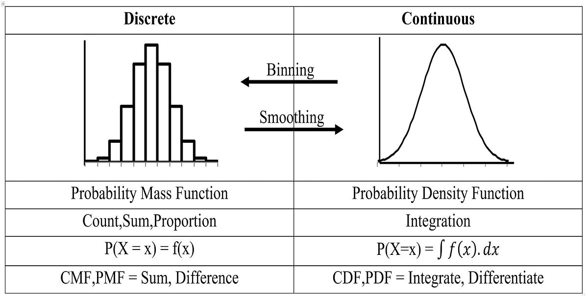
Probability Mass Function
The probability mass function (PMF) is a concept used in probability theory to describe the probability distribution of a discrete random variable.
It assigns probabilities to each possible value that the random variable can take.
For a discrete random variable X, the probability mass function is defined as:
$$P(X = x)$$
where P(X = x) represents the probability that X takes on the specific value x.
Properties of Probability Mass function
Non-negative probabilities: The probabilities assigned by the PMF are non-negative, meaning that P(X = x) ≥ 0 for all possible values of x.
The sum of probabilities: The sum of probabilities over all possible values of the random variable is equal to 1. Mathematically, Σ P(X = x) = 1, where the sum is taken over all possible values of x.
Probability of a specific value: The probability of a specific value x is given by P(X = x). This represents the likelihood that the random variable takes on that value.
ILLUSTRATION
Probability distributed to discrete values

Cumulative Distribution Function for PMF
The Cumulative distribution function for PMF is a concept used in probability theory to describe the probability distribution of a discrete random variable.
It provides the cumulative probability of the random variable being less than or equal to a specific value.
$$F(x) = P(X ≤ x)$$
where F(x) represents the probability that X is less than or equal to x.
Probability Density Function
The probability density function (PDF) is a concept used in probability theory and statistics to describe the probability distribution of a continuous random variable.
The PDF indicates the "density" of probability at different points along the range of the random variable.
Higher values of the PDF at a particular point suggest a higher likelihood of the random variable taking on values around that point.
$$∫ f(x) dx$$
where the integration is performed over the entire range of x.

Properties of the Probability density function
Non-negative values: The PDF is always non-negative, meaning that f(x) ≥ 0 for all x.
Integration over the entire range: The area under the PDF curve over the entire range of possible values is equal to 1. Mathematically, ∫ f(x) dx = 1, where the integration is performed over the entire range of x.
Probability calculation over intervals: The probability of the random variable falling within a specific interval [a, b] is given by the integral of the PDF over that interval. Mathematically, P(a ≤ X ≤ b) = ∫[a, b] f(x) dx.
Cumulative Distribution Function for PDF
The Cumulative distribution function for PdF is a concept used in probability theory to describe the probability distribution of a continuous random variable.
It provides the cumulative probability of the random variable being less than or equal to a specific value.
$$F(x) = P(X ≤ x) = ∫_{-∞}^{x} f(t) dt$$
Properties of Cumulative distribution function
Non-decreasing: The CDF increases or stays constant as the value of x increases. Mathematically, if a ≤ b, then F(a) ≤ F(b).
Bounds: The CDF is bounded between 0 and 1. That is, 0 ≤ F(x) ≤ 1 for all x.
Common types of Discrete probability distribution
Bernoulli Distribution
Binomial Distribution
Multinomial Distribution
Bernoulli Distribution
The Bernoulli distribution is a discrete probability distribution that models a single trial with two possible outcomes: success and failure.
FORMULA
$$P(X = k) = p^k * (1 - p)^(1 - k)$$
where,
X is the random variable representing the outcome of a single Bernoulli trial
k is the specific outcome (either 0 or 1)
p is the probability of success.
The probability mass function (PMF) of the Bernoulli distribution can be defined as follows:
$$P(X = 1) = p (probability of success)$$
$$P(X = 0) = 1 - p (probability of failure)$$
where X is the random variable that represents the outcome of the trial, taking the value 1 for success and 0 for failure.

Mathematical Example
Let us assume that out of every 50 people in a city, 1 is a business owner. So, If one citizen is selected randomly, what is the distribution of business owners?
Solution:
Given:
p = 1/50
w.k.t
$$P (X = x) = p*(1-p)^(1-x)$$
Thus,
$$P (X = x) = (1/50) * (1 – 1/50)^(1-x)$$
Let us compute for x = 0, 1
If, x = 1
$$p(X = 1) = 1/50 = 0.02$$
If, x = 0
$$p(X = 0) = q = 1 – p = 1 – 1/50 = 49/50 = 0.98$$
Thus, the probability of success, i.e., the selected citizen being a business owner, is 0.02, and the probability of failure, i.e., the selected citizen not being a business owner, is 0.98.
APPLICATION
Modeling binary events: The Bernoulli distribution is used to model binary events or situations where there are only two possible outcomes, such as success/failure, yes/no, or heads/tails.
Binary classification problems: In machine learning and statistics, the Bernoulli distribution is used in binary classification problems, where the goal is to predict whether an instance belongs to one of two classes based on a set of features.
Risk analysis: The Bernoulli distribution can be used to model and analyze risks, where success represents an event of interest (e.g., occurrence of an accident) and failure represents its absence.
Behavioral studies: The Bernoulli distribution can be applied in behavioral studies to model individual choices or responses that have only two possible outcomes.
Binomial distribution
The binomial distribution is a discrete probability distribution that models the number of successes in a fixed number of independent Bernoulli trials.
FORMULA
$$P(X = k) = C(n, k) * p^k * (1 - p)^(n - k)$$
where,
X is the random variable representing the number of successes.
k is a specific number of successes (0 ≤ k ≤ n)
C(n, k) is the binomial coefficient (n choose k)
$$C(n, k) = n! / (k! * (n - k)!)$$
p is the probability of success in each trial
(1 - p) is the probability of failure.
ILLUSTRATION
Probability of success for 20 trails.

Mathematical Example
80% of people who purchase pet insurance are women. If 9 pet insurance owners are randomly selected, find the probability that exactly 6 are women.
Solution:
Given
p=0.8
n=9
k=6
w.k.t
$$P(X = k) = C(n, k) * p^k * (1 - p)^(n - k)$$
After calculation we get
$$p(exactly-6women)=0.176$$
Multinomial distribution
The multinomial distribution is a discrete probability distribution that generalizes the concept of the binomial distribution to situations with more than two categories or outcomes.
It models the number of occurrences of each category in a fixed number of independent trials.
FORMULA

ILLUSTRATION
Probability of success for A, B, C classes

Common types of Continuous probability distribution
Normal Distribution
Log-Normal Distribution
Chi-square Distribution-Test
Student's T Distribution-Test
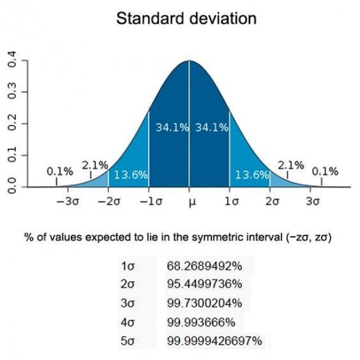
Normal Distribution
A normal distribution, also known as a Gaussian distribution or a bell curve, is a continuous probability distribution that is symmetric and characterized by its mean and standard deviation.
In a normal distribution, the data points are symmetrically distributed around the mean, forming a bell-shaped curve.
The mean represents the center of the distribution.
The standard deviation determines the spread or dispersion of the data points around the mean.
FORMULA

Where
x is the variable
μ is the mean
σ is the standard deviation

Log-Normal Distribution
The log-normal distribution is a continuous probability distribution of a random variable whose logarithm follows a normal distribution.
It is often used to model variables that are inherently positive and skewed, such as stock prices, incomes, or sizes of populations.

FORMULA

***NOTE***
The log-normal distribution is specifically designed to model variables that are positively skewed, where the logarithm of the variable follows a normal distribution.
Student's T distribution-Test
The Student's t-distribution, also known as the t-distribution, is a continuous probability distribution that arises in statistics and is widely used in hypothesis testing and constructing confidence intervals when the sample size is small or when the population standard deviation is unknown.
FORMULA
The formula is for hypothesis testing
$$t = (x̄ - μ) / (s / √n)$$
where,
x̄ (x-bar) represents the sample mean
μ (mu) represents the hypothesized mean
s (s) represent the sample standard deviation
n represent the sample size
ILLUSTRATION

***NOTE***
Small Sample Size: The t-distribution is especially useful when working with small sample sizes (typically less than 30).
Chi-square Distribution-Test
The chi-square distribution test, also known as the chi-square test, is a statistical method used to assess the association between categorical variables or to test the goodness-of-fit of observed data to an expected distribution.
The chi-square test involves comparing the observed frequencies in different categories with the expected frequencies based on a specified null hypothesis.
FORMULA
The formula is for hypothesis testing

ILLUSTRATION

***we will look at hypothesis testing in an upcoming blog***
TRANSFORMATION
Transformation involves applying mathematical functions to modify the distribution or relationship between variables.
TYPES
Common transformations include,
Logarithmic
Exponential
Square root
Power transformations
Logarithmic transformation
- The logarithmic transformation applies the logarithm function to the data values. It is often used to reduce the effect of extreme values and make the data distribution more symmetric.
Logarithmic transformations are especially useful when the data exhibits exponential growth or when the range of values is large.
$$y = log_b(x)$$
EXAMPLE
Applying the natural logarithm (ln) to a positively skewed variable can help make the distribution more symmetrical.
ILLUSTRATION

Exponential Transformation
- The exponential transformation raises the data values to an exponent. It is useful for counteracting the compressing effect of the logarithm or emphasizing exponential growth patterns in the data.
$$y = e^x$$
EXAMPLE
Raising the data values to a power greater than 1 can accentuate higher values and highlight exponential relationships.
ILLUSTRATION

Square Root Transformation
The square root transformation takes the square root of the data values.
It is effective in reducing the impact of extreme values and making the data distribution more symmetric.
Square root transformations are commonly used when dealing with count data (e.g., number of occurrences, number of customers) with a non-linear relationship.
$$y = sqrt(x)$$
EXAMPLE
Taking the square root of the count of occurrences of an event can help normalize the distribution.
Power Transformation
Power transformations involve raising the data values to a power other than 1.
They can be used to manipulate the data distribution, make it more linear, or address issues such as heteroscedasticity.
$$y = x^p$$
What is heteroscedasticity?
CONCLUSION
In conclusion, this blog has provided a concise yet comprehensive overview of probability and statistics in data science. We have explored key concepts, techniques, and real-world applications, highlighting the power of numbers in uncovering insights and making informed decisions. Armed with this knowledge, you are now equipped to navigate the exciting realm of data science with confidence.
Hope enjoyed !!!
Support the blog !!!
Thankyou !!!