Mastering Logistic Regression: A Mathematical Journey to Predictive Excellence
INTRODUCTION
Logistic regression, similar to linear regression, is a powerful statistical technique used for modeling the relationship between a dependent variable and independent variables. However, while linear regression is primarily used for continuous and numerical target variables, logistic regression is specifically designed for binary classification problems, where the target variable has two possible outcomes.
TYPES OF LOGISTIC REGRESSION
Binomial Logistic Regression
Multinomial Logistic Regression
Ordinal Logistic Regression
FORMULA
$$σ(z) = 1 / (1 + e^(-z))$$
where:
σ(z) is the probability of the positive class (or the probability of y = 1).
z is the linear combination of the independent variables and their corresponding coefficients, given by:
$$z = β0 + β1x1 + β2x2 + ... + βnxn$$
Here:
β₀, β₁, β₂, ..., βₙ are the coefficients or parameters of the logistic regression model.
x₁, x₂, ..., xₙ are the values of the independent variables.
ODDS FUNCTION
The odds of an event happening (p) can be expressed as the ratio of the probability of the event occurring to the probability of the event not occurring.
$$Odds(p) = p / (1 - p)$$
Here:
Odds(p) represents the odds of the event happening.
p is the probability of the event occurring.
LOGIT + REGRESSION=LOGISTIC REGRESSION
Let's see how Logistic regression came from the odds function and Linear regression.
LOGIT FUNCTION:
The logarithmic odds function gives out the Logit function Y
Equation 1:
$$Y=ln(odds)\ \ \ Y=ln(p(x)/1-p(x))$$
Equation 2:
Based on number of variables in the dataset we will use Y
SIMPLE LINEAR REGRESSION (OR) MULTIPLE LINEAR REGRESSION EQUATION:
$$Y = β0 + βx$$
or
$$Y=β0 + β1x1 + β₂x₂ + ... + βnxn$$
From above equations
$$ln(p(x)/1-p(x))=β₀ + βx$$
or
$$ln(p(x)/1-p(x))=β0 + β1x1 + β2x2 + ... + βnxn$$
Exponentiation
$$e^(ln(p(x)/1-p(x)))=e^(β0 + βx)$$
or
$$e^(ln(p(x)/1-p(x)))=e^(β0 + β1x1 + β2x2 + ... + βnxn)$$
By formula e^(ln(x))=x
$$p(x)/1-p(x)=e^(β0 +βx)$$
or
$$p(x)/1-p(x)=e^(β0 + β1x1 + β2x2 + ... + βnxn)$$
Let Y=e^(β₀ +βx) or Y=e^(β₀ + β₁x₁ + β₂x₂ + ... + βₙxₙ)
Now
$$p(x)=Y(1-p(x))$$
$$Y=p(x)+Yp(x)$$
Taking p(x) common
$$Y=p(x)(1+Y)$$
Rearrange
$$p(x)=Y/(1+Y)$$
Substitute for Y
$$p(x)=e^(β0 + βx)/(1+e^(β0 + βx))$$
or
$$p(x)=e^(β0 + β1x1 + β2x2 + ... + βnxn)/(1+e^(β0 + β1x1 + β2x2 + ... + βnxn))$$
Let z=β₀ + βx or z=e^(β₀ + β₁x₁ + β₂x₂ + ... + βₙxₙ)
Now equation becomes
$$p(x)=e^z/(1+e^z)$$
Or
$$p(x)=1/(e^(-z)+1)$$
Hence the above p(x) is the equation of logistic regression.
EXAMPLE MATHEMATICAL PROBLEM
The student dataset has an entrance mark based on historic data of those who are selected or not selected. Given that parameter values are β₀=1 and β=8.
SOLUTION:
Let p(z) be the probability that the student select or not based on the mark
if p(z)>=0.5 selected
else not selected
W.K.T
$$p(z) = 1 / (1 + e^(-z))$$
here
$$z=β₀ + βx$$
Substitute given values
$$z=481$$
$$p(x)=1/(1+e^(-481)$$
we get
$$p(x)=0.44$$
conclusion,
p(x)=0.44<0.5 the student will not get selected
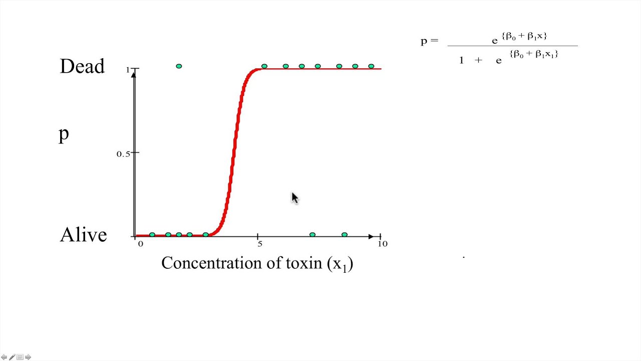
BINARY LOGISTIC REGRESSION
Binary logistic regression is a statistical technique used to model the relationship between a set of independent variables and a binary (two-class) categorical dependent variable. It is a type of logistic regression specifically designed for binary classification problems.
EXAMPLE
Based on the concentration of toxin the people alive or dead
CODE
import numpy as np
from sklearn.linear_model import LogisticRegression
from sklearn.preprocessing import StandardScaler
from sklearn.metrics import accuracy_score

# Create a manual dataset
X = np.array([[2.0],
              [3.5],
              [4.0],
              [2.5],
              [3.0],
              [3.5]])
y = np.array([0, 1, 1, 0, 1, 0])

# Standardize the features
scaler = StandardScaler()
X_scaled = scaler.fit_transform(X)

# Create a LogisticRegression object for binary logistic regression
logreg = LogisticRegression()

# Fit the model on the data
logreg.fit(X_scaled, y)

# Predict the classes for the data
y_pred = logreg.predict(X_scaled)

# Calculate the accuracy of the model
accuracy = accuracy_score(y, y_pred)
print('predicted values',y_pred)
print("Accuracy:", accuracy)
OUTPUT
predicted values [0 1 1 0 0 1]
Accuracy: 0.6666666666666666
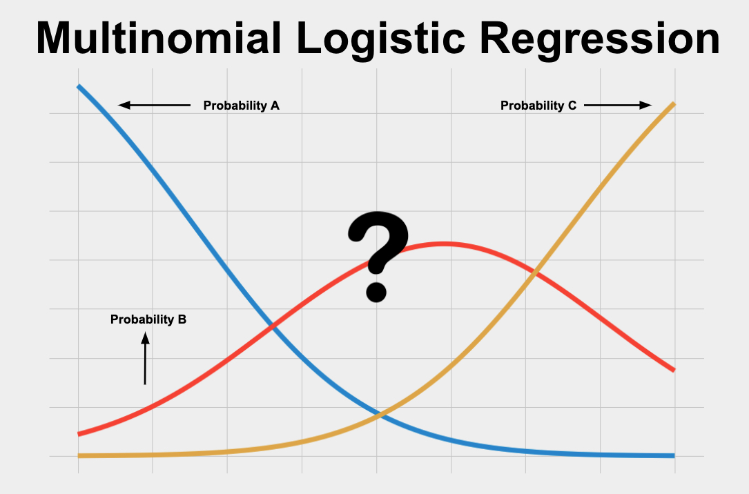
MULTINOMIAL LOGISTIC REGRESSION
A multinomial regression model, also known as multinomial logistic regression, is a statistical technique used to model the relationship between multiple independent variables and a categorical dependent variable with more than two categories.
It is an extension of binary logistic regression, specifically designed for multiclass classification problems.
EXAMPLE
Dataset with more than two classes
Let A, B, and C be the classes
CODE
import numpy as np
from sklearn.linear_model import LogisticRegression
from sklearn.preprocessing import StandardScaler
from sklearn.metrics import accuracy_score

# Create a manual dataset
X = np.array([[2.0, 1.0],
              [3.5, 1.5],
              [4.0, 1.0],
              [2.5, 0.5],
              [3.0, 1.5],
              [3.5, 0.5]])
y = np.array([0, 1, 2, 0, 1, 2])

# Standardize the features
scaler = StandardScaler()
X_scaled = scaler.fit_transform(X)

# Create a LogisticRegression object for multinomial logistic regression
logreg = LogisticRegression(multi_class='multinomial')

# Fit the model on the data
logreg.fit(X_scaled, y)

# Predict the classes for the data
y_pred = logreg.predict(X_scaled)

# Calculate the accuracy of the model
accuracy = accuracy_score(y, y_pred)
print("predicted values",y_pred)
print("Accuracy:", accuracy)
OUTPUT
predicted values [0 1 2 0 1 2]
Accuracy: 1.0
ORDINAL LOGISTIC REGRESSION
Ordinal logistic regression, also known as proportional odds model or cumulative logit model, is a statistical technique used to model the relationship between independent variables and an ordinal categorical dependent variable. It is an extension of logistic regression designed specifically for ordinal outcome variables with ordered categories.
EXAMPLE
Used for datasets having ordinal values in the output column
example:
high=0.8,medium=0.4,low=0

CODE
import numpy as np
from mord import LogisticIT
from sklearn.preprocessing import StandardScaler
from sklearn.metrics import accuracy_score

# Create a manual dataset for ordinal logistic regression
X = np.array([[2.0],
              [3.5],
              [4.0],
              [2.5],
              [3.0],
              [3.5]])
y = np.array([0, 1, 2, 0, 1, 2])

# Standardize the features
scaler = StandardScaler()
X_scaled = scaler.fit_transform(X)

# Create a LogisticIT object for ordinal logistic regression
logreg_ordinal = LogisticIT()

# Fit the model on the data
logreg_ordinal.fit(X_scaled, y)

# Predict the classes for the data
y_pred_ordinal = logreg_ordinal.predict(X_scaled)

# Calculate the accuracy of the model
accuracy_ordinal = accuracy_score(y, y_pred_ordinal)
print("predicted values",y_pred_ordinal)
print("Ordinal Logistic Regression Accuracy:", accuracy_ordinal)
OUTPUT
predicted values [0 2 2 0 1 2]
Ordinal Logistic Regression Accuracy: 0.8333333333333334
NOTE:
Certainly! In real-world datasets, logistic regression for classification tasks typically involves additional steps such as data cleaning, data transformation, and model selection based on the number of output classes.
Data Cleaning: Real-world datasets often contain missing values, outliers, or inconsistencies. Before implementing logistic regression, it is crucial to clean the data by handling missing values, removing outliers, and addressing any data quality issues.
Data Transformation: Logistic regression assumes that the input data is numeric and follows certain assumptions (e.g., linearity, no multicollinearity). Therefore, it may be necessary to transform the data by encoding categorical variables, standardizing numeric features, or applying other transformations to meet the assumptions of the model.
Model Selection: Logistic regression is suitable for binary classification problems. However, if the dataset has multiple output classes, you may need to consider alternative approaches. For example:
For binary classification (2 classes), binary logistic regression can be used.
For multi-class classification (more than 2 classes), you can choose between:
- Multinomial logistic regression, which extends binary logistic regression to handle multiple classes directly.
The choice of the model depends on factors such as the nature of the problem, dataset size, class imbalance, and computational considerations.
By considering these additional steps, you can effectively handle real-world datasets, clean and transform the data appropriately, and choose the most suitable logistic regression model for the classification task at hand.
ORDINAL VS BINOMIAL VS MULTINOMIAL
| Logistic Regression Type | Dependent Variable | Number of Classes | Relationship Modeled | Assumptions |
| Ordinal Logistic Regression | Ordinal (Ordered) | Three or more | Probability of falling into or above a category | Proportional odds assumption |
| Binomial Logistic Regression | Binary | Two | Probability of belonging to a specific class | Independent observations, Linearity |
| Multinomial Logistic Regression | Nominal (Unordered) | Three or more | Probability of belonging to each class | Independence, Linearity, No multicollinearity |
CONCLUSION
Logistic regression is a versatile tool for classification tasks, allowing us to model relationships between independent variables and categorical outcomes. Understanding the differences between binomial, multinomial, and ordinal logistic regression can help in selecting the appropriate approach based on the nature of the problem and the number of output classes.
HOPE YOU ENJOYED READING IT!!!
STAY TUNED !!!
SUPPORT MY BLOG !!!
THANKYOU!!!