Optimizing Performance: The Journey of Gradient Descent in Logistic Regression


INTRODUCTION
Welcome to our blog on optimizing performance in logistic regression through the power of gradient descent! In this article, we dive into the inner workings of the cost function and its relationship with the popular optimization algorithm. Join us as we unravel the secrets behind achieving accurate predictions and efficient convergence in logistic regression models.
COST FUNCTION
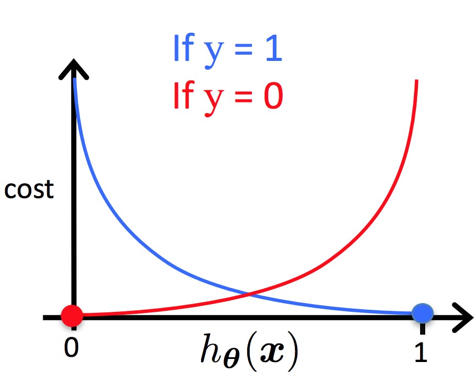
The cost function for logistic regression is commonly known as the "logistic loss" or "log loss."
It is a mathematical representation of the error between the predicted probabilities and the actual class labels in a binary classification problem.
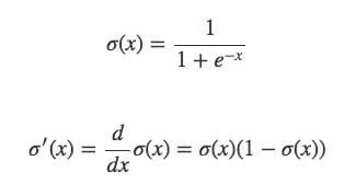
The cost function uses the sigmoid function to map the linear regression output to a probability between 0 and 1.
By minimizing the cost function using techniques like gradient descent, we can effectively train the logistic regression model to make accurate predictions.
LOG LOSS -FORMULA
L = (-1/m) * Σ [ y(i) * log(y_hat(i)) + (1 - y(i)) * log(1 - y_hat(i)) ]
Where:
L represents the cost function.
m is the total number of training examples.
Σ denotes the sum over all training examples.
y(i) represents the actual class label (0 or 1) for the i-th training example.
y_hat(i) is the predicted label.
log denotes the natural logarithm
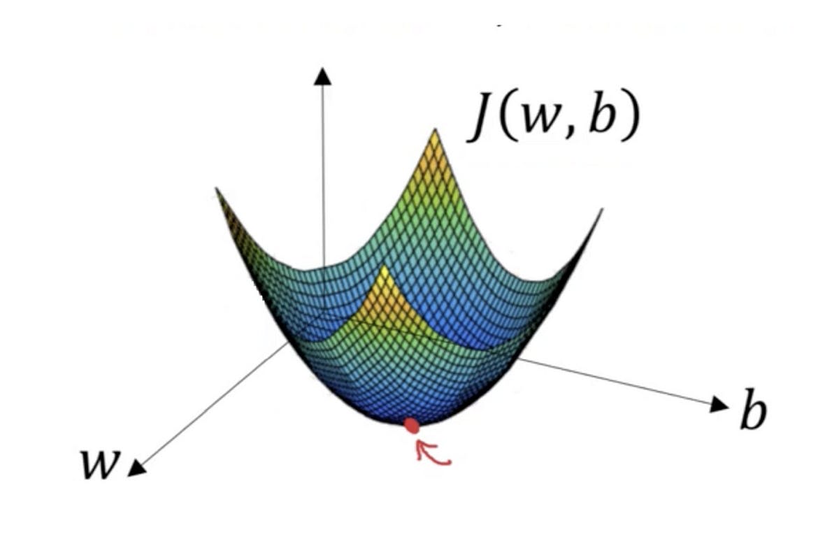
GRADIENT DESCENT FOR COST FUNCTION
$$W=W-(lr)*dL/dW$$
Where,
W represents the weight parameters of the logistic regression model.
lr denotes the learning rate, which is a hyperparameter that controls the step size in each iteration of gradient descent.
dL/dW represents the derivative of the cost function with respect to the weights. It indicates the direction and magnitude of the steepest descent, guiding the update of the weights (known as gradient).
DERIVING GRADIENT FOR LOGISTIC REGRESSION
Suppose we have mxn data points**(INPUTS)**
Let x
X = [  [x11  x12  x13  ...  x1n]
       [x21  x22  x23  ...  x2n]
       [x31  x32  x33  ...  x3n]
       ...   ...   ...  ...  ...
       [xm1  xm2  xm3  ...  xmn]
]
We have n number of labeled outputs
Let y
y = [  [y1]
       [y2]
       [y3]
        ...
       [yn]
   ]
After prediction, we have n number of predicted output
Let y_hat
y_hat = [  [y_hat1]
           [y_hat2]
           [y_hat3]
             ...
           [y_hatn]
]
Step 1: w.k.t y_hat1 = σ(w0 + w1x1 + w2x2 + ... + wnxn)
similarly
y_hat = [ [σ(w0 + w1x11 + w2x22 + ... + wnx1n)]
      [σ(w0 + w1x21 + w₂x22 + ... + wnx2n)]
      [σ(w0 + w1x31 + w₂x32 + ... + wnx3n)]
       ...
      [σ(w0 + w1xm1 + w2xm2 + ... + wnxmn)]
]
Step 2: By Dot product and scalar multiplication rule in matrix
we derive
y_hat=σ(WX)
Step 3: Substitute y_hat in Log loss
L = (-1/m) * [ y * log(σ(WX)) + (1 - y) * log(1 - σ(WX)) ]
Step 4: find dL/dW
Find first half
$$d(y*log(y_hat)/dW$$
By applying the chain rule for above
for example Derivative of L with respect to y_hat and y_hat with respect to W,
$$dL/dw=dL/d(y_hat)*d(y_hat)/dL$$
Now the first half becomes
Equation _________________(1):
$$d(ylog(yhat)/dW=y(1-y_hat)X$$
Step 5:similarly apply the chain rule for
w.k.t y_hat=σ(WX)
$$d((1 - y) * log(1 - y_hat))/dW$$
in step4 step5 we used this formula which is mentioned below,
we get,
Equation__________________(2):
$$d((1 - y) * log(1 - y_hat))dW = -yhat(1-y)X$$
Step 6: From equations 1 and 2 the step3 equation becomes
$$dL/dW=-1/m(y(1-yhat)-yhat(1-y))X$$
Step 7: By expanding and canceling
we obtained GRADIENT
$$dL/dW=-1*(y-yhat)X/m$$
Step 8: updating weights
$$W=W+(lr)*(y-yhat)X/m$$
IMPLEMENTING GRADIENT DESCENT FOR LOGISTIC REGRESSION
import numpy as np
def gradient_descent_logistic_regression(X,y,learning_rate,epochs):

     #we have to add 1 at 0th column as shown in step2 in derivation
    X=np.insert(X,0,1,axis=1)
    #weights
    w=np.ones(X.shape[1])
    #learning rate
    lr=learning_rate
    for i in range(epochs):
        #Step 1: w.k.t y_hat1 = σ(w0 + w1x1 + w2x2 + ... + wnxn)
       # Calculate predicted probabilities using sigmoid function
        y_hat=sigmoid(np.dot(X,weights))
        # W=W+(lr)*(y-yhat)X/m
        weights=weights+lr*(np.dot((y-yhat),X)/X.shape[0])
        #returning coefficients and intercept
        return weights[1:],weights[0]
def sigmoid(z):
    return 1/(1+np.exp(-z))
CONCLUSION
In conclusion, we explored the power of gradient descent in optimizing performance for logistic regression. By leveraging the gradient descent algorithm, we can iteratively update the weights and minimize the cost function to improve the accuracy of our logistic regression model. Understanding the cost function and its connection to the sigmoid activation function is crucial in this process. Through this blog, we've gained insights into the inner workings of logistic regression and how gradient descent enhances its predictive capabilities, ultimately enabling us to make more accurate and reliable predictions in binary classification tasks.
PRE-REQUISITE
Costfunction for linear regression
Hope you enjoyed learning !!!
Stay tuned !!!
Thankyou !!!